California Housing Valuation: A Geo-XAI Approach

Integrating GIS Feature Engineering with Explainable AI

Overview

This project builds a robust real estate valuation model for the California housing market by fusing Geospatial Analysis with Machine Learning.

Unlike traditional models that treat coordinates merely as numbers, this approach engineers specific spatial features—specifically the geodesic distance to the nearest coastline—to capture the non-linear economic value of “location.” Furthermore, the project moves beyond the “black box” of prediction by utilizing SHAP (SHapley Additive exPlanations) to visualize exactly how geography impacts price.

Key Features

• GIS Engineering: Topology repair and coordinate reprojection (EPSG:4326 $\to$ EPSG:3310) for accurate meter-based distance calculations.
• High-Performance ML: Utilized XGBoost to capture complex, non-linear relationships, achieving an $R^2$ score of ~0.82.
• Explainable AI (XAI): Deployed SHAP values to quantify the marginal contribution of spatial features.
• Interactive Visualization: Generated a Folium heatmap to visualize the “Location Premium” (positive vs. negative spatial impact) across the state.

Methodology

1. Data Acquisition & Cleaning

The dataset is sourced from the Hands-On Machine Learning repository. Initial steps involved handling missing values and preparing the raw dataframe.

2. GIS Feature Engineering

Raw Lat/Lon coordinates are insufficient for identifying “coastal proximity.”

• Reprojection: Converted data to California Albers (EPSG:3310) to measure distance in meters rather than degrees.
• Topology Repair: Applied .buffer(0) to fix self-intersections in the California coastline polygon.
• Calculation: Computed the precise distance from every property to the nearest point on the coast.

3. Predictive Modeling

An XGBoost Regressor was trained on the enriched dataset.

• Input Features: Median Income, Housing Median Age, Rooms, Population, Distance to Coast (Engineered), etc.
• Performance: The model achieved an $R^2$ of 0.8187 on the test set.

4. Explainable AI (SHAP)

We used TreeExplainer to calculate SHAP values, allowing us to see:

• Global Importance: Which features drive prices the most?
• Local Interpretation: How much does “being 5km from the coast” add to a specific house’s value?

Results & Visualisations

1. Feature Importance (SHAP Beeswarm)

The SHAP summary plot reveals that Median Income and Distance to Coast are the primary drivers of housing prices.

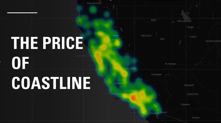
2. The “Location Premium” Map

We visualised the spatial heterogeneity of housing value.

• Red Areas: Positive location premium (e.g., Coastal zones, Bay Area).
• Blue Areas: Negative location impact (e.g., Inland/Central Valley).

💡 Insights

• Proximity Matters: The engineered feature dist_to_coast_km proved to be a top-tier predictor, significantly improving model performance compared to using raw coordinates alone.
• Non-Linearity: The relationship between distance and price is not linear; prices drop sharply within the first 10-20km from the coast, which XGBoost captured effectively.